OpenZFS 2.1 released – let’s talk about its brand new dRAID vdevs – Bestgamingpro

By Patrick Centeno Last updated Jul 3, 2021

Enlarge / OpenZFS has added distributed RAID topologies to its toolkit with the current release of 2.1.Zero.

Aurich Lawson

Friday afternoon, the OpenZFS adventure published 2.1.Zero model of our favorite “it’s fancy, but surely the price” filesystem. The brand new release is compatible with FreeBSD 12.2-RELEASE and later, and Linux kernels Three.10-5.13. This launch offers a number of core efficiency improvements, in addition to a few entirely new, primarily enterprise-focused options and various extraordinarily superior usage instances.

Right away, we’ll focus on arguably the most important feature provided by OpenZFS 2.1.Zero: the dRAID vdev topology. dRAID has been growing rapidly since at least 2015 and reached beta status when merged into OpenZFS getting started in November 2020. Since then it has been under close scrutiny in a number of leading growth OpenZFS retailers, meaning that at present the launch is ‘new’ for manufacturing, and not “new” as in the untested case.

Understanding Distributed RAID (dRAID)

In case you already thought ZFS topology was a fancy topic, get carried away. Distributed RAID (dRAID) is a brand new vdev topology that we first encountered during a presentation at the OpenZFS Dev Summit 2016.

When creating a dRAID vdev, the administrator specifies a lot of information, parity and hotspare sectors per band. These figures are not biased against the variety of precise drives within the vdev. We can see this in motion in the following example, taken from the foundational ideas of RAID. Documentation:

[email protected]:~# zpool create mypool draid2:4d:1s:11c wwn-Zero wwn-1 wwn-2 ... wwn-A
[email protected]:~# zpool standing mypool

  pool: mypool
 state: ONLINE
config:

        NAME                  STATE     READ WRITE CKSUM
        tank                  ONLINE       Zero     Zero     Zero
          draid2:4d:11c:1s-Zero  ONLINE       Zero     Zero     Zero
            wwn-Zero             ONLINE       Zero     Zero     Zero
            wwn-1             ONLINE       Zero     Zero     Zero
            wwn-2             ONLINE       Zero     Zero     Zero
            wwn-Three             ONLINE       Zero     Zero     Zero
            wwn-Four             ONLINE       Zero     Zero     Zero
            wwn-5             ONLINE       Zero     Zero     Zero
            wwn-6             ONLINE       Zero     Zero     Zero
            wwn-7             ONLINE       Zero     Zero     Zero
            wwn-Eight             ONLINE       Zero     Zero     Zero
            wwn-9             ONLINE       Zero     Zero     Zero
            wwn-A             ONLINE       Zero     Zero     Zero
        spares
          draid2-Zero-Zero          AVAIL

DRAID topology

In the example above, we have eleven disks: wwn-Zero through wwn-A. We have created a single dRAID vdev with 2 parity gadgets, four information gadgets, and 1 spare gadget per band – in condensed parlance, one draid2:Four:1.

Although we have eleven complete records in the draid2:Four:1, only six are used in each information band — and one in each physical Bandaged. In a world of good vacuums, frictionless surfaces, and spherical chickens, the disk format of a draid2:Four:1 would look something like this:

Zero	1	2	Three	Four	5	6	7	Eight	9	A
s	P	P	re	re	re	re	P	P	re	re
re	s	re	P	P	re	re	re	re	P	P
re	re	s	re	re	P	P	re	re	re	re
P	P	re	s	re	re	re	P	P	re	re
re	re	.	.	s	.	.	.	.	.	.
.	.	.	.	.	s	.	.	.	.	.
.	.	.	.	.	.	s	.	.	.	.
.	.	.	.	.	.	.	s	.	.	.
.	.	.	.	.	.	.	.	s	.	.
.	.	.	.	.	.	.	.	.	s	.
.	.	.	.	.	.	.	.	.	.	s

With success, dRAID takes the idea of “diagonal parity” RAID a step further. The primary parity RAID topology was not RAID5 – it was RAID3, where parity was on a hard drive and fast, rather than being distributed throughout the array.

RAID5 removed the fixed parity drive and distributed parity across all disks in the array instead, which provided considerably faster random write operations than the conceptually less complicated RAID3 because it did not clog every write to a hard and fast parity disk.

dRAID takes this idea – spread parity across all disks, rather than bundling everything onto one or two attached disks – and expands it to spares. If a disk fails in a dRAID vdev, the parity and information sectors that lived on the lifeless disk are copied to the reserved spare sector (s) for each affected tape.

Let’s take the simplified diagram above and investigate what happens if we fail a disk out of the array. The preliminary failure leaves holes in many information teams (in this simplified diagram, scratches):

Zero	1	2	Four	5	6	7	Eight	9	A
s	P	P	re	re	re	P	P	re	re
re	s	re	P	re	re	re	re	P	P
re	re	s	re	P	P	re	re	re	re
P	P	re	re	re	re	P	P	re	re
re	re	.	s	.	.	.	.	.	.

However, after resilvering, we do this on the reserve capacity previously reserved:

Zero	1	2	Four	5	6	7	Eight	9	A
re	P	P	re	re	re	P	P	re	re
re	P	re	P	re	re	re	re	P	P
re	re	re	re	P	P	re	re	re	re
P	P	re	re	re	re	P	P	re	re
re	re	.	s	.	.	.	.	.	.

Please note that these diagrams are simplified. The total image includes teams, slices, and rows, which we won’t attempt to address here. The logical format can also be swapped randomly to distribute problems more evenly across the disks, primarily based on offset. These in the hairiest details are inspired to take a look at this detail comment in the single code commit.

It’s also worth noting that dRAID requires fixed bandwidths, not the dynamic widths supported by conventional RAIDz1 and RAIDz2 vdevs. If we are using 4kn disks, a draid2:Four:1 vdev, just like the one proven above, would require 24KB on disk for each metadata block, whereas a typical six-width RAIDz2 vdev would only want 12KB. This gap will get worse as the values of d+p obtain a draid2:Eight:1 would require a whopping 40KiB for a similar metadata block!

For this reason, the particular vdev allocation could be very useful in pools with dRAID vdevs-when a pool with draid2:Eight:1 and a three-large particular must detailing a metadata block of 4KiB, it does so in just 12KiB on the particular, instead of 40KiB on the draid2:Eight:1.

Efficiency, fault tolerance and recovery dRAID

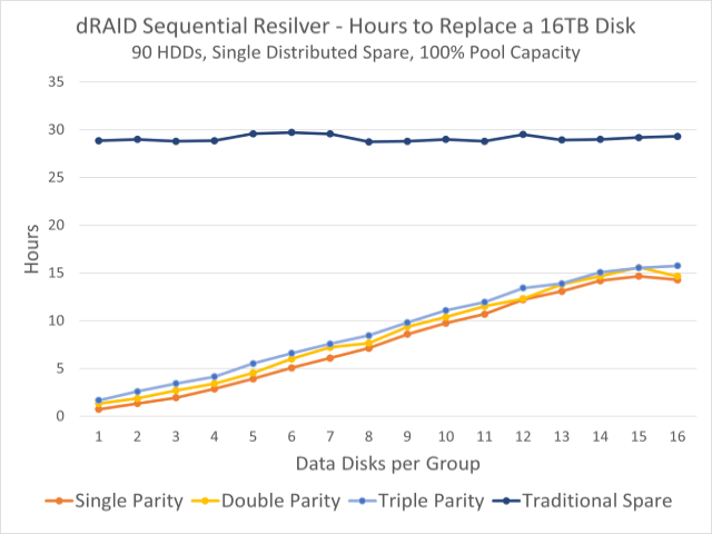
This graph shows the resilvering times observed for a pool of 90 disks. The dark blue line at the top corresponds to the resilvering time on a fixed hotspare disk; the colored lines below show the resilvering times on the distributed reserve capacity. — This graph reveals notable resilvering opportunities for a pool of 90 drives. The dark blue line at the top is the time of resilvering on a hard and fast hot spare; the colorful varieties below present opportunities to replenish distributed spare capacity.

For almost half of them, a vdev dRAID will also apply to an equal group of conventional vdevs, for example, a draid1:2:Zero on 9 disks will perform almost equivalent to a pool of three three-width RAIDz1 vdevs. Fault tolerance can also be linked – you are guaranteed to survive a single outage with p=1, just as you might be with RAIDz1 vdevs.

Find out that we have declared fault tolerance to be Related, not an identical one. A standard three-wide RAIDz1 vdev pool is just guaranteed to survive a single drive failure, but will most likely survive a second, as long as the second failed drive is not part of the same vdev as the primary, all chunks are nice.

In a nine discs draid1:2, a second disk failure will almost actually kill the vdev (and the pool with it), if this failure occurs before resilvering. Since there are no teams attached for particular person tapes, a second drive failure could be very likely to destroy other sectors in already degraded tapes, regardless of which the disk fails second.

This somewhat reduced fault tolerance is offset by considerably faster resilvering opportunities. In the graphic at the top of this part, we will see that in a pool of ninety 16 TB disks, resilvered on a spare takes about thirty hours, regardless of how we configured the vdev dRAID, but resilvering on distributed standby capacity can take as little as an hour.

This is largely because resilvering on a distributed hot spare distributes the write load among all surviving disks. When resilvering on a spare, the hot spare itself is the bottleneck: reads come from all disks in the vdev, but all writes must be done by the hot spare. However, when resilvering to a distributed spare capacity, each and write workloads are distributed among all surviving disks.

The distributed resilver can also be a sequential resilver, rather than a therapeutic resilver, which means that ZFS can simply copy to all affected sectors, regardless of what blocks these sectors belong. Therapeutic resilvers, on the other hand, should analyze the entire block tree, which leads to a random learning workload, rather than a sequential learning workload.

When a bodily replacement of the failed disk is added to the pool, this resilvering operation will be therapeutic, not sequential, and it will hamper the write efficiency of a single replacement disc, rather than that of the full vdev. However, the time to complete this operation is much less, because vdev is simply not in a degraded state to begin with.

Conclusion

Distributed RAID vdevs are primarily intended for large storage servers — OpenZFS draid much of the design and testing revolved around 90-disc techniques. On a smaller scale, vdevs and spares remain as helpful as they have ever been.

We especially caution those new to storage to be careful with draid– it is a considerably more advanced format than a pool with classic vdevs. The quick resilvering is amazing, however draid succeeds in every compression range and in a few efficiency situations because of its essentially fixed length bands.

As conventional discs grow larger without significant efficiency increasing, draid and its quick resilvering could get fascinating even on smaller techniques, but it will surely take some time to accurately determine where the candy begins. In the meantime, keep in mind that RAID is just not a backup and the features draid!